System Identification & Finite Element Analysis

1. Kinematic vs. Dynamic Modeling

Standard robotic control systems rely on Kinematic Models. Kinematic models calculate motion based solely on geometry and joint angles, operating under the assumption that the machine's physical links are perfectly rigid. This approach fails under real-world industrial conditions, where machines move at high speeds, manipulate heavy payloads and suffer normal usage wear and tear. Then, structural deflection and vibration occur, rendering kinematic assumptions inaccurate.

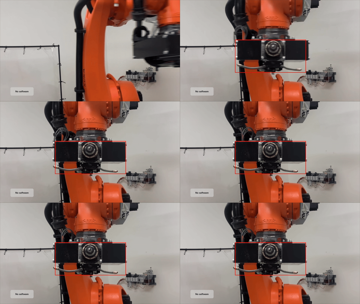
Excessive vibration on a robot arm end effector, using its original kinematic control.

Reforge Robotics utilizes a dynamic model, backed by the Finite Element Method (FEM). Our dynamic FEM model calculates motion by incorporating the physical forces acting upon the machine, including inertia, payload mass, and material elasticity. Instead of assuming absolute rigidity, the FEM engine segments the machine's structure into smaller elements, to compute exact physical deformations. This allows the control software to predict and account for structural bending and vibration, and act preemptively before they impact operational precision.

2. Mechanical Systems

Every machine operates according to fundamental laws of physics. To dictate (and improve!) machine behavior using software, physical phenomena such as inertia, structural flexibility, and friction must be translated into math. The fundamental equation used for this translation from real-world to math, is the Equation of Motion (EoM).

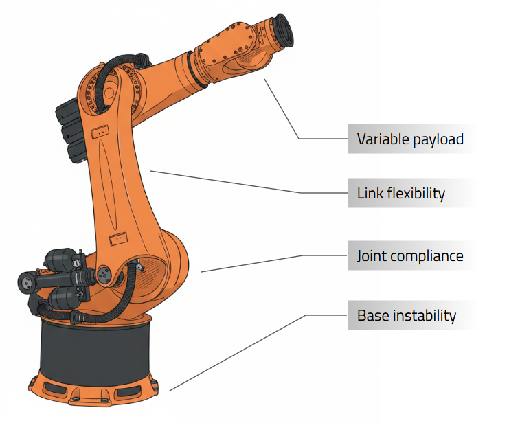
Relevant mechanical characteristics of a robot arm, neglected by kinematic control.

An EoM functions as a dynamic blueprint. While standard CAD models define static geometry, an EoM defines dynamic physical reactions. It establishes the exact relationship between the forces applied to a machine by its motors and the resulting real-world movement.

Consider a simple robotic arm. The EoM calculates not only the intended joint rotations, but also the unintended physical realities: the micro-flexing of the physical links under payload stress, the resistance of the joints, and the continuous influence of gravity on the structure.

3. Equations of Motion

The most fundamental representation of mechanical dynamics used to construct an EoM is the spring-mass-damper system. Complex industrial machines, including multi-axis robots, are modeled as networks of these basic interactive elements.

• Mass ($m$): Represents the object's weight and resistance to acceleration (inertia).
• Stiffness ($k$): Represents the structure's resistance to bending or deformation, acting like a spring.
• Damping ($c$): Represents energy dissipation within the system, such as joint friction or internal material yielding.

The dynamic behavior of this basic system is governed by a standard differential equation:

In this equation, $x$, $\dot{x}$, and $\ddot{x}$ represent the position, velocity, and acceleration of the machine component, respectively. $F(t)$ represents the external forces applied over time, such as motor torque.

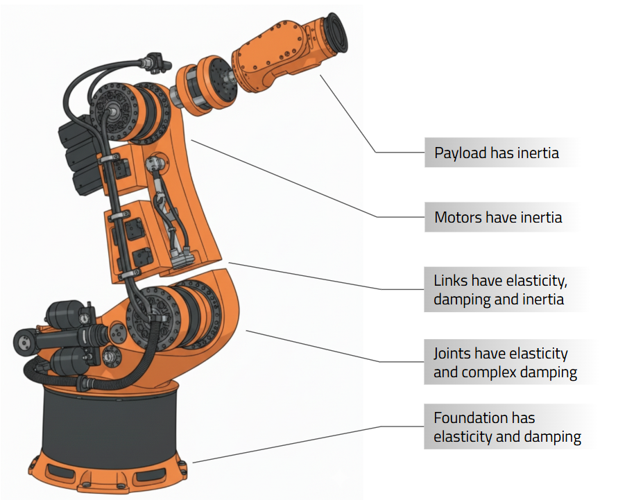
Relevant physical effects considered by our model.

By converting physical reality into an EoM, our control software predicts exactly how the machine will move, bend, and vibrate under its specific conditions. This mathematical prediction is required to implement preemptive physics-based control before physical actuation occurs.

4. Experimental Data and System Identification

Theoretical parameter values for mass ($m$), stiffness ($k$), and damping ($c$) are insufficient for high-precision control. Manufacturing tolerances, assembly variations, and material degradation cause real-world physical values to deviate from initial engineering estimates. Precise parameter determination requires empirical data.

Our system identification routine isolates the machine's exact dynamic profile. Sensors capture real-time physical responses while specific motor commands actuate the machine across a designated spectrum of frequencies. These controlled excitations trigger the latent mechanical behaviors of the system, exposing exact resonant frequencies and structural flex points.

The collected sensor data is processed to construct a graphical representation of the machine's EoM. This representation is the frequency response function (FRF). An FRF maps exactly how the physical structure amplifies or suppresses movement at specific operational conditions and frequencies.

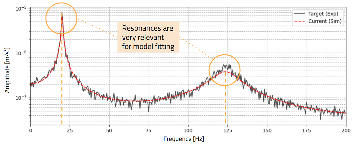
Frequency response function (FRF) showing the amplitude of the model prediction (red line) and the real machine data (black line).

Through FRF and other analyses, the precise physical characteristics of the machine are mathematically mapped. This empirical mapping provide the baseline for our system identification.

5. Parameter Optimization

We start our model calibration with baseline estimates for mass, stiffness, and damping. Computational algorithms iteratively adjust these theoretical parameters to match reality, via AI-based optimization routines. The objective is exact alignment, when the digital FRF of the model converge with the empirical FRF derived from the physical sensor data.

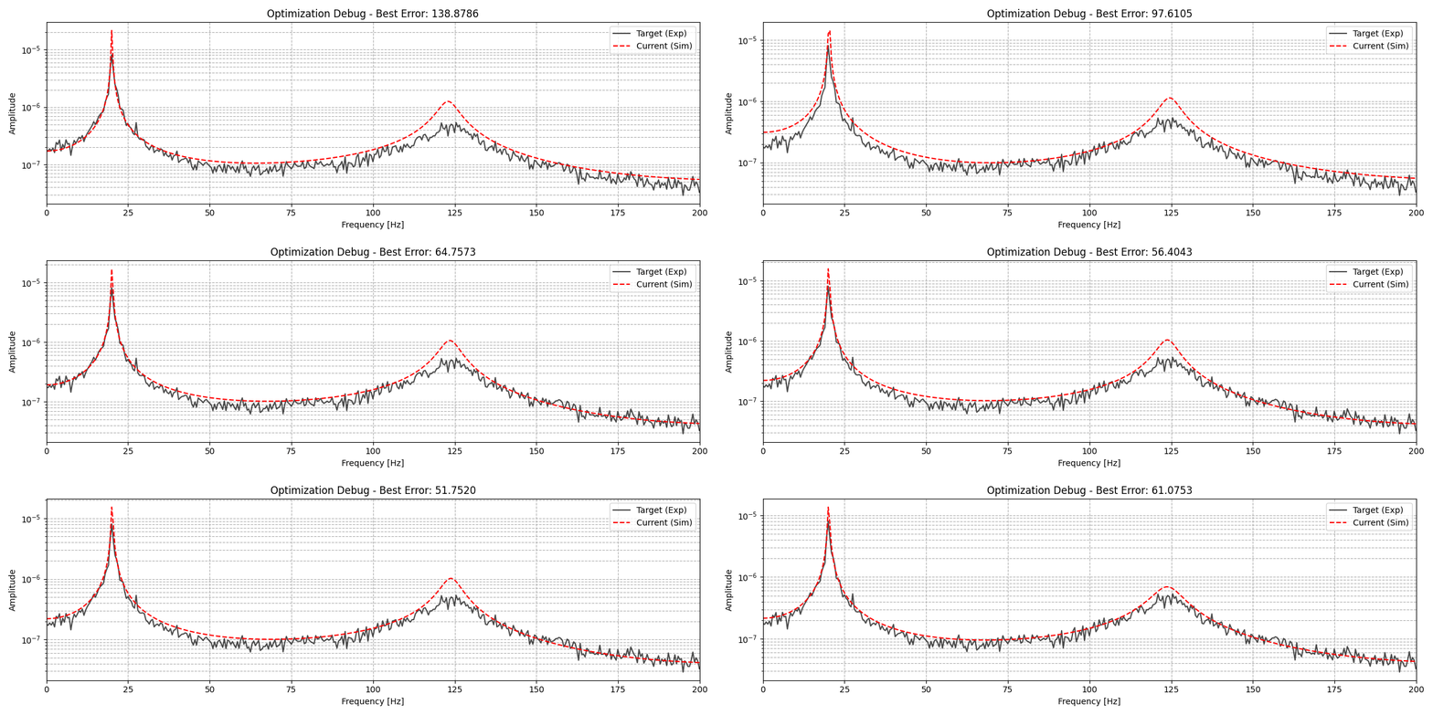
Progression of the FRF convergence process during optimization, showing the amplitude of the model prediction (red line) and the real machine data (black line).

Optimization terminates when the exact physical parameters are determined, and both digital and experimental FRFs match. The model functions as a trustworthy digital representation of the physical machine. This convergence completes the system identification, and ensures a representative and reliable model of the robot has been found.

6. Model-Based Control

The calibrated dynamic model is then deployed directly into the control architecture. This methodology is defined as model-based control. The software processes the exact mathematical replica to anticipate and neutralize physical deviations before hardware actuation occurs.

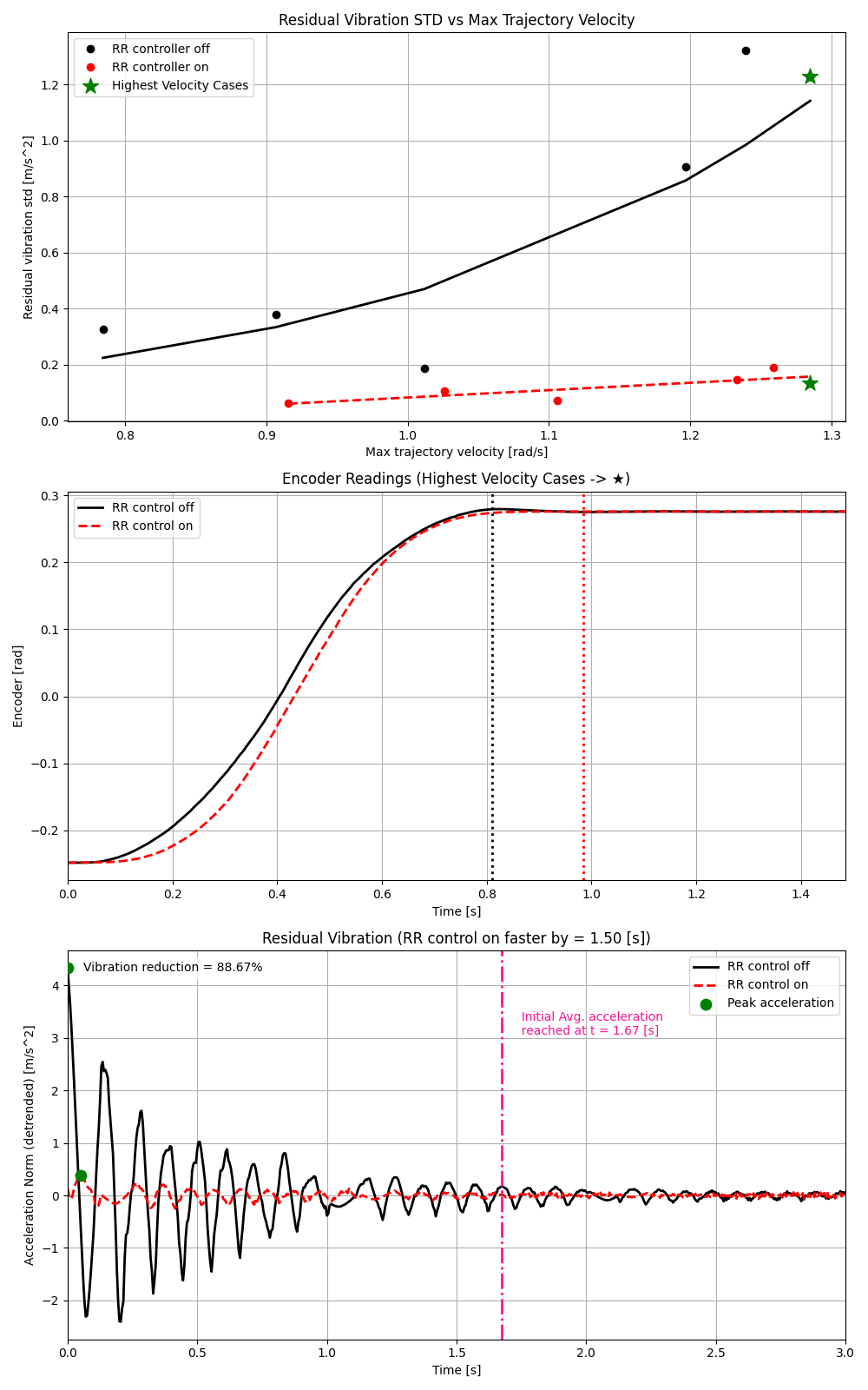
Full behavioral comparison, with Reforge Robotics vibration control (red line) vs. original kinematic control (black line). 1. Top image shows the vibration vs. velocity, where the robot is able to achieve higher velocities with less vibration using vibration control; 2. Middle image shows the encoder measurement for the fastest achievable velocity for both, illustrating an increase in productivity with vibration control without any overshoot, and; 3. Bottom plot shows the vibration time signal comparison, illustrating overall 85% reduction of vibration even with the 2x productivity increase (defined as when the kinematic control reaches the same vibration level as the vibration control).

The model calculates optimal outputs for vibration suppression and precise trajectory tracking. Machine precision, acceleration limits, and operational velocity increase strictly through software execution. Hardware remains unmodified. This is software that gives robots superpowers.

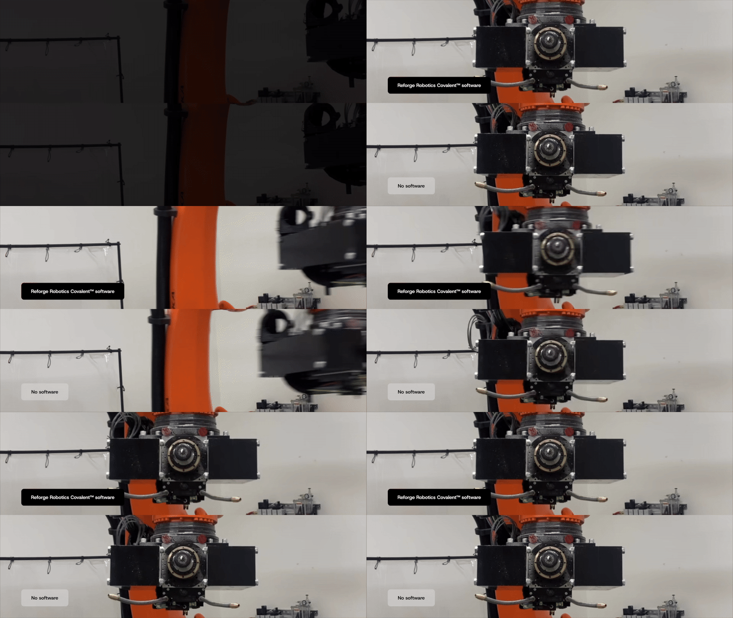
Comparison of the vibration on a robot arm end effector, using original kinematic control vs. Reforge Robotics Covalent software.