Control

Use Joint Tracker during runtime by loading the identified joint-controller model bundle, computing an optimized joint command, and sending that command to the robot manufacturer's SDK.

Before using this page, complete Calibration and Identification so that src/robot/models/current/joint_tracker contains the identified Joint Tracker model bundle.

Inputs

The Joint Tracker controller needs:

• The controller sample time, in seconds.
• The identified model folder, usually src/robot/models/current/joint_tracker.
• The desired joint position trajectory in radians.
• The number of robot joints and model-backed axes.

The robot SDK is still responsible for executing the optimized command on the robot.

Example 1: Full Known Trajectory

Use this path when the full joint trajectory is known before the move starts. This example is ideal for short and repeatable trajectories.

python
import numpy as np
import robot_sdk  # Replace with the SDK package for the robot you are using.
from reforge_core.control.joint_tracker import JointTrackerInterface

sample_time_s = 0.004
model_directory = "src/robot/models/current/joint_tracker"
num_joints = 6

# Initialize Joint Tracker with the identified model bundle.
initializing_JTC = JointTrackerInterface(
    sample_time=sample_time_s,
    num_joints=num_joints,
    model_directory=model_directory,
    num_axes=6,
)

# Replace this line with the desired joint trajectory from your planner or robot SDK.
desired_trajectory_rad = np.asarray(robot_sdk.get_planned_joint_trajectory())

# Optimize the complete desired trajectory before sending it to the robot.
JTC_offline_mode = initializing_JTC.process_trajectory(
    command=desired_trajectory_rad,
)

# Send the optimized command with your robot SDK.
robot_sdk.send_joint_trajectory(
    positions=JTC_offline_mode.positions,
    velocities=JTC_offline_mode.velocities,
    accelerations=JTC_offline_mode.accelerations,
    sample_time=sample_time_s,
)

Example 2A: Stream a Known Full Trajectory

Use this path when the full trajectory is known before execution, but you want Joint Tracker to optimize and emit command windows while the robot is already moving. This way, you do not need to wait until the whole trajectory is optimized. This example is ideal for applications where the trajectory is known beforehand but is very long.

python
import numpy as np
import robot_sdk  # Replace with the SDK package for the robot you are using.
from reforge_core.control.joint_tracker import JointTrackerInterface

sample_time_s = 0.004
model_directory = "src/robot/models/current/joint_tracker"
num_joints = 6

# Initialize Joint Tracker with the identified model bundle.
initializing_JTC = JointTrackerInterface(
    sample_time=sample_time_s,
    num_joints=num_joints,
    model_directory=model_directory,
    num_axes=6,
)

# Replace this line with the full desired joint trajectory from your planner.
desired_trajectory_rad = np.asarray(robot_sdk.get_planned_joint_trajectory())

# Create the stream-mode controller and append the complete known trajectory.
JTC_stream_mode = initializing_JTC.process_trajectory_stream_mode()
JTC_stream_mode.append_reference(desired_trajectory_rad)

# Tell Joint Tracker that no more desired samples will be appended.
JTC_stream_mode.finish()

# Start optimizing command windows in the background.
JTC_stream_mode.start()

# Consume optimized command windows and send each window to the robot SDK.
while not JTC_stream_mode.is_complete():
    command_window = JTC_stream_mode.pop()
    if command_window is None:
        break

    robot_sdk.send_joint_trajectory(
        positions=command_window.positions,
        velocities=command_window.velocities,
        accelerations=command_window.accelerations,
        sample_time=sample_time_s,
    )

JTC_stream_mode.close()

Example 2B: Stream an Online Trajectory

Use this path when the path and trajectory generation are done while the robot is moving or performing a task. You can append new desired samples as your planner/trajectory generation creates them.

python
import numpy as np
import robot_sdk  # Replace with the SDK package for the robot you are using.
from reforge_core.control.joint_tracker import JointTrackerInterface

sample_time_s = 0.004
model_directory = "src/robot/models/current/joint_tracker"
num_joints = 6

# Initialize Joint Tracker with the identified model bundle.
initializing_JTC = JointTrackerInterface(
    sample_time=sample_time_s,
    num_joints=num_joints,
    model_directory=model_directory,
    num_axes=6,
)

# Create the stream-mode controller.
JTC_online_mode = initializing_JTC.process_trajectory_stream_mode()

# Append the first desired samples before starting the stream.
desired_trajectory_beginning_rad = np.asarray(
    robot_sdk.get_next_desired_joint_samples()
)
JTC_online_mode.append_reference(desired_trajectory_beginning_rad)

# Start optimizing command windows in the background.
JTC_online_mode.start()

# Real-time loop: each iteration feeds JTC the planner's latest samples and
# sends one optimized command window to the robot. It exits once JTC has
# optimized and drained every sample you appended.
while not JTC_online_mode.is_complete():
    # YOUR PLANNER: append new desired samples whenever your planner produces
    # them. When it has nothing new (e.g. a pause between moves), skip the
    # append and JTC keeps holding the last desired sample until more arrive.
    if robot_sdk.has_new_desired_joint_samples():
        new_desired_samples_rad = np.asarray(
            robot_sdk.get_next_desired_joint_samples()
        )
        JTC_online_mode.append_reference(new_desired_samples_rad)

    # YOUR PLANNER: once no more samples will ever be appended, tell JTC to wind
    # down so the loop can finish. finish() does not stop the JTC but it let it
    # know that your path planner will no longer generate new samples.
    if robot_sdk.planner_is_finished():
        JTC_online_mode.finish()

    # JTC: take the next optimized command window. pop() blocks until a window
    # is ready and returns None only after the stream is finished and drained.
    command_window = JTC_online_mode.pop()
    if command_window is None:
        break

    # YOUR ROBOT SDK: send the optimized command window to the robot.
    robot_sdk.send_joint_trajectory(
        positions=command_window.positions,
        velocities=command_window.velocities,
        accelerations=command_window.accelerations,
        sample_time=sample_time_s,
    )

# JTC: release the background optimizer thread when you are done.
JTC_online_mode.close()

Runnable Repository Example

The minimal snippets above show only the controller usage. The full simulation example, including trajectory generation, plotting, diagnostics, and expected results, is available in:

bash
src/robot/example_usage/joint_tracker/joint_tracker_example_usage.py

Run it from the repository root with:

bash
python3 src/robot/example_usage/joint_tracker/joint_tracker_example_usage.py

Expected Output

Running the example prints RMS tracking-error summaries to the console and renders two figures.

Figure 1 — Robot commands

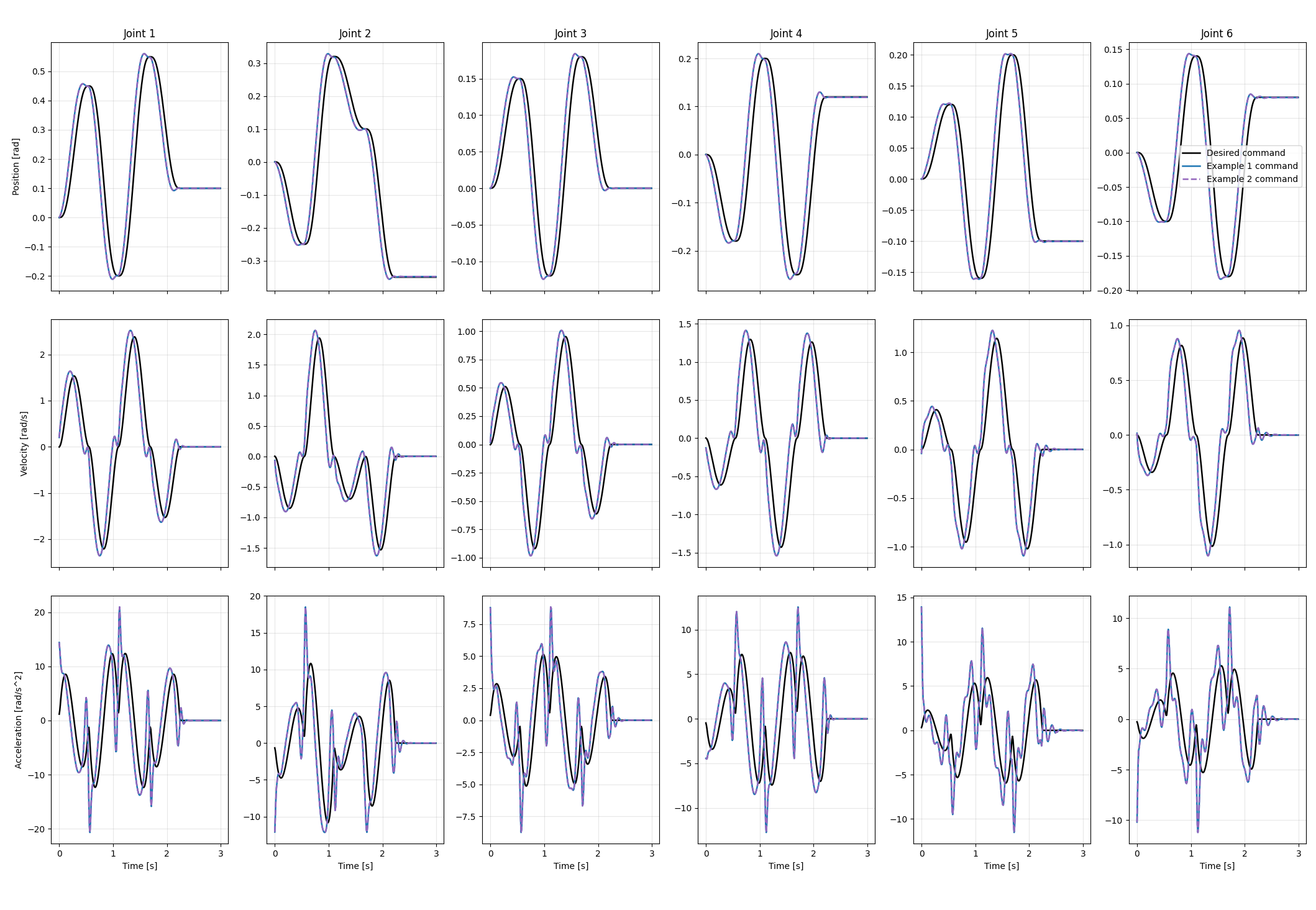
This figure shows the joint commands sent to the robot. It is laid out as a grid: one column per joint, and three rows — position [rad], velocity [rad/s], and acceleration [rad/s²]. Three commands are overlaid on every subplot:

• Desired command (black, solid): the raw reference trajectory you want the robot to follow.
• Example 1 command (blue, solid): the command JTC optimizes from the fully known trajectory (Example 1 / stream mode).
• Example 2 command (purple, dashed): the command JTC optimizes online, as the planner streams samples in (Example 2B).

The key takeaway is that the optimized commands deliberately differ from the desired command — JTC pre-shapes the position, velocity, and acceleration profiles to counteract each joint's flexible dynamics. The Example 1 and Example 2 commands overlap almost exactly, confirming that the online (streamed) path reproduces the offline result.

Figure 2 — Robot response

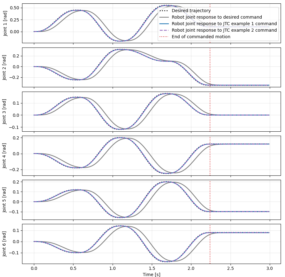
This figure shows the resulting robot motion — the simulated plant response to each command — with one subplot per joint (position [rad] versus time):

• Desired trajectory (black, dotted): the reference the joint should track.
• Response to desired command (gray): how the joint actually moves when the raw desired command is sent directly. Note the overshoot and residual oscillation, most visible after the motion ends.
• Response to JTC Example 1 command (blue) and Response to JTC Example 2 command (purple, dashed): how the joint moves when driven by the JTC-optimized commands. Both track the desired trajectory closely with strongly suppressed vibration.
• The red dotted vertical line marks the end of the commanded motion; the residual vibration is what happens to the right of it, during the final dwell.

Together the figures tell the whole story: JTC changes the command (Figure 1) so that the robot's actual response (Figure 2) follows the desired trajectory with far less vibration than commanding the desired trajectory directly. The RMS tracking-error values printed to the console quantify that improvement.